자료구조
데이터를 효율적으로 저장하고 관리하며 처리하기 위한 방법
적절한 자료구조를 선택하면 프로그램의 성능을 크게 향상시킬 수 있다
ADT(추상 자료형, Abstract Data Type)
데이터와 그 데이터에 대한 연산을 추상적으로 정의한 것
예를들어 Stack 이라는 ADT는 데이터를 쌓고(push) 빼는(pop) 동작을 할 수 있다
내부적으로 배열을 사용하든, 리스트를 사용하든 상관없다. 사용자는 '쌓고 빼는' 기능만 알면 된다
효율적인 자료구조인지 평가하는 두가지 요소
시간복잡도 (Time complexity) - 얼마나 빨라?
공간복잡도 (Space complexity) - 메모리를 얼마나 적게 사용했어?
복잡도를 표현하는 방법
Big Oh (O): 알고리즘이 절대로 특정 시간 이상 걸리지 않는다는 것을 보장합니다. (상한)
Big Ω (Ω): 알고리즘이 적어도 특정 시간 이상 걸린다는 것을 보장합니다. (하한)
Big Θ (Θ): 알고리즘이 실제로 특정 시간 정도 걸린다는 것을 의미합니다. (상한과 하한이 일치)
보편적으로 Big-O (Big Oh) 표기법을 사용
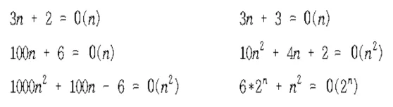

O(1) < O(log N) < O(N) < O(N logN) < O(N^2) < O(N^3) < O(2^N) < O(N!)
(N : 데이터의 개수)
Stack(스택)
LIFO (Last-In First-Out / 후입 선출) 구조
삽입과 삭제가 항상 제일 뒤(최근) 요소에서 이루어진다. 그리고 가장 최근에 삽입한 요소를 top이라고 지칭한다
Stack 구현연습
Python
import numpy as np

# Stack 을 배열로 구현해보자
class STACK:
  def __init__(self, max_size):
    self.data = np.zeros(max_size, dtype=np.int32)
    self.max_size = max_size
    self.top = 0

  def is_empty(self):
    return self.top == 0

  def is_full(self):
    return self.top == self.max_size

  def push(self, value):
    if self.is_full():
      print("Stack is full.")
      return

    self.data[self.top] = value
    self.top += 1

  def pop(self):
    if self.is_empty():
      print("Stack is empty.")
      return

    self.top -= 1
    return self.data[self.top]

# 위에서 만든 STACK 을 사용해서 자료를 넣고 빼기 테스트
stack_test = STACK(10)

for i in range(1, 11):
  stack_test.push(i)

stack_test.push(11)

while not stack_test.is_empty():
  print(stack_test.pop(), end=" ")
print()

stack_test.pop()
Stack is full.
10 9 8 7 6 5 4 3 2 1
Stack is empty.
멀티스레드에 안전한 스택
import numpy as np
import threading
import time
import random

# 스레드에 안전한 Stack
class STACK:
  def __init__(self, max_size):
    self.data = np.zeros(max_size, dtype=np.int32)
    self.max_size = max_size
    self.top = 0
    self.lock = threading.Lock()

  def is_empty(self):
    with self.lock:
      return self.top == 0

  def is_full(self):
    with self.lock:
      return self.top == self.max_size

  def push(self, value):
      if self.is_full():
        print("Stack is full.")
        return

      with self.lock:
        self.data[self.top] = value
        self.top += 1

  def pop(self):

    if self.is_empty():
      print("Stack is empty.")
      return

    with self.lock:
      self.top -= 1
      return self.data[self.top]


def push_thread(stack, num_size):
  for i in range(num_size):
    value = random.randint(1, 100)
    stack.push(value)
    print(f"Thread {threading.current_thread().name}: Pushed: {value}")
    time.sleep(0.01)

def pop_thread(stack):
  time.sleep(0.01)
  while not stack.is_empty():
    value = stack.pop()
    print(f"Thread {threading.current_thread().name}: Popped {value}")
    time.sleep(0.01)

test_stack = STACK(20)

push_thread_1 = threading.Thread(target=push_thread, args=(test_stack, 10), name="PushThread1")
push_thread_2 = threading.Thread(target=push_thread, args=(test_stack, 10), name="PushThread2")

pop_thread_1 = threading.Thread(target=pop_thread, args=(test_stack,), name="PopThread1")
pop_thread_2 = threading.Thread(target=pop_thread, args=(test_stack,), name="PopThread2")

push_thread_1.start()
push_thread_2.start()
pop_thread_1.start()
pop_thread_2.start()

push_thread_1.join()
push_thread_2.join()
pop_thread_1.join()
pop_thread_2.join()

print("Done")
Thread PushThread1: Pushed: 11
Thread PushThread2: Pushed: 33
Thread PushThread2: Pushed: 5
Thread PopThread1: Popped 5Thread PushThread1: Pushed: 41
Thread PopThread2: Popped 41
Thread PushThread2: Pushed: 39
Thread PushThread1: Pushed: 10
Thread PopThread1: Popped 10
Thread PopThread2: Popped 39
Thread PushThread2: Pushed: 10
Thread PushThread1: Pushed: 43
Thread PopThread1: Popped 43Thread PopThread2: Popped 10
Thread PushThread2: Pushed: 42
Thread PushThread1: Pushed: 68
Thread PopThread2: Popped 68Thread PopThread1: Popped 42
Thread PushThread2: Pushed: 62
Thread PushThread1: Pushed: 87
Thread PopThread1: Popped 87
Thread PopThread2: Popped 62
Thread PushThread2: Pushed: 16
Thread PushThread1: Pushed: 39
Thread PopThread1: Popped 39
Thread PopThread2: Popped 16
Thread PushThread2: Pushed: 37
Thread PushThread1: Pushed: 48
Thread PopThread1: Popped 48
Thread PopThread2: Popped 37
Thread PushThread2: Pushed: 78
Thread PushThread1: Pushed: 85
Thread PopThread1: Popped 85
Thread PopThread2: Popped 78
Thread PushThread2: Pushed: 94
Thread PushThread1: Pushed: 91
Thread PopThread1: Popped 91
Thread PopThread2: Popped 94
Thread PopThread1: Popped 33
Thread PopThread2: Popped 11
Done
Queue (큐)
FIFO(First-In First-Out / 선입 선출) 구조
놀이공원이나 은행의 대기줄처럼 먼저 들어온 요소를 먼저 내보낸다
큐 구현연습
import numpy as np

# Queue 구현해보기
class QUEUE:
  def __init__(self, max_size):
    self.data = np.zeros(max_size, dtype=np.int32)
    self.max_size = max_size
    self.front = 0
    self.rear = 0
    self.size = 0

  def is_empty(self):
    return self.size == 0

  def is_full(self):
    return self.size == self.max_size

  def enqueue(self, item):
    if self.is_full():
      print("Queue is Full")
      return False

    self.data[self.rear] = item
    self.rear = (self.rear + 1) % self.max_size
    self.size += 1
    return True

  def dequeue(self):
    if self.is_empty():
      print("Queue is Empty")
      return None

    item = self.data[self.front]
    self.front = (self.front + 1) % self.max_size
    self.size -= 1
    return item
# 큐 테스트
q_test = QUEUE(10)
res = []
# 1~11 추가
# 11 추가 실패
for i in range(1, 12):
q_test.enqueue(i)
# 1~6 까지 dequeue
# 남은 수는 7~10, 4개
for _ in range(6):
n = q_test.dequeue()
if n is not None:
res.append(n)
# 12~18 추가 7개
# 남은공간 6개이니까 18은 추가 실패
for i in range(12, 19):
q_test.enqueue(i)
# 11개 dequeue
# 10개의 데이터가 있으니 1번 실패
for _ in range(11):
n = q_test.dequeue()
if n is not None:
res.append(n)
print(res)Queue is Full
Queue is Full
Queue is Empty
[1, 2, 3, 4, 5, 6, 7, 8, 9, 10, 12, 13, 14, 15, 16, 17]
Array(배열)
배열은 연속된 메모리 공간에 같은 타입의 데이터를 순차적으로 저장하는 구조
인덱스를 통해 빠르게 접근 가능 하나.. 데이터 중간 삽입과 삭제시에는 효율적이지 않다
Linked List
생성 후 자유롭게 원소를 추가/삭제할 수 있는 자료구조
기본적으로는 하나의 요소에 그 다음 요소가 연결되어 있는 단순 연결리스트의 형태로 구현되고 경우에 따라 원형 연결 리스트, 이중 연결 리스트 등으로 나타내기도 한다

[주의] 파이썬의 List는 Linked List가 아니라 dynamic array 로 구현되어있다고 한다
Single Linked List 구현해보기
Python
# Linked List 구현해보자 (Single)
class MyLinkedList:
  class Node:
    def __init__(self, data):
      self.data = data
      self.next = None

  def __init__(self):
    self.head = None
    self.size = 0

  def __str__(self):
    cur_node = self.head
    result = ""
    while cur_node is not None:
      result += str(cur_node.data) + " "
      cur_node = cur_node.next
    return result

  def get_size(self):
    return self.size

  def is_empty(self):
    return self.size == 0

  def access(self, index):
    if index < 0 or index >= self.size:
      print("index out of range")
      return None

    cur_node = self.head
    for _ in range(index):
      cur_node = cur_node.next
    return cur_node.data

  def append(self, data):
    new_node = self.Node(data)

    if self.is_empty():
      self.head = new_node
    else:
      cur_node = self.head
      while cur_node.next is not None:
        cur_node = cur_node.next
      cur_node.next = new_node

    self.size += 1

  def insert(self, index, data):
    if index < 0 or index > self.size:
      print("index out of range")
      return False

    new_node = self.Node(data)

    if index == 0:
      new_node.next = self.head
      self.head = new_node
    else:
      cur_node = self.head
      for i in range(index - 1):
        cur_node = cur_node.next
      new_node.next = cur_node.next
      cur_node.next = new_node

    self.size += 1
    return True

  def delete(self, index):
    if index < 0 or index >= self.size:
      print("index out of range")

    if index == 0:
      self.head = self.head.next
    else:
      cur_node = self.head
      for _ in range(index - 1):
        cur_node = cur_node.next
      cur_node.next = cur_node.next.next

    self.size -= 1
# Linked List 테스트
my_list = MyLinkedList()
for i in range(1, 11):
  my_list.append(i)
print(my_list)

for i in range(5):
  my_list.delete(i)
print(my_list)

my_list.insert(my_list.get_size(), 11)
my_list.append(12)
print(my_list)

for i in range(5):
  my_list.insert(i * 2, i * 2 + 1)
print(my_list)
1 2 3 4 5 6 7 8 9 10
2 4 6 8 10
2 4 6 8 10 11 12
1 2 3 4 5 6 7 8 9 10 11 12
Hash Table (해시테이블)
키-값 쌍으로 데이터를 저장하는 자료구조
해시함수를 사용하여 키를 인덱스로 변환하고, 이 해시 값을 배열의 인덱스로 사용하여 데이터를 저장하고 검색한다
ex) 파이썬의 dict
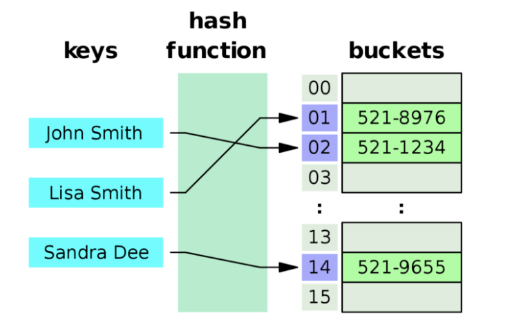
서로 다른 키가 같은 해시 값을 갖는 경우 해시 충돌이라고 한다
충돌 처리 방법에는 Separate Chaining 과 Open Addressing 방법이 있다
Separate Chaining : 같은 해시 값을 가진 데이터를 연결 리스트로 연결하는 방법
Open Addressing : 충돌 발생 시 빈 공간을 찾아 데이터를 저장하는 방법
- 탐색방법 : Linear Probing, Quadratic Probing, Double Hashing
장점 : 빠른 검색, 삽입, 삭제 (평균 시간 복잡도 O(1))
단점 : 충돌 발생 시 성능 저하, 해시 테이블 크기 조정의 어려움, 순서가 보장되지 않음
해시 테이블은 순서가 중요하지 않고 빠른 검색 속도가 요구되는 상황에 적합
Binary Tree
각 노드가 최대 두 개의 자식 노드를 갖는 계층적 자료 구조
가장 위에 있는 노드를 Root 노드라고 한다
자식 노드가 없는 노드를 leaf node 라고 한다

Linear Search
선형검색, 순차탐색, 전탐색
데이터가 저장된 배열을 처음부터 끝까지 순차적으로 탐색하여 원하는 값을 찾는 방법
장점: 단순, 구현이 쉽다. 데이터가 정렬되어 있지 않아도 된다
단점: 비효율적이다. 데이터의 양이 많을 경우 검색 시간이 오래걸린다.
시간복잡도
- 최악의 경우 : O(N) (N은 배열의 크기)
- 평균적인 경우 : O(N)
- 최선의 경우 : O(1) (찾는 값이 배열의 첫 번째 요소일 경우)
Binary Search (이진 탐색)
정렬된 데이터에서 특정 값을 찾을 때 사용하는 탐색 방법
탐색 범위를 절반씩 줄여나가면서 목표 값을 찾는다
시간복잡도
- 최악의 경우 : O(log n) (n은 배열의 크기)
- 평균적인 경우 : O(log n)
- 최선의 경우 : O(1) (찾는 값이 배열의 중간에 있을 경우)
이진탐색 구현연습
Python
# binary search를 구현해보자

def binary_search(arr, value):
    low = 0
    high = len(arr) - 1

    while low <= high:
        center = (low + high) // 2
        if arr[center] == value:
            return True
        elif arr[center] < value:
            low = center + 1
        else:
            high = center - 1

    return False
narr = [1, 3, 5, 7, 9]
def check(value):
res = binary_search(narr, value)
if res == True:
print(f'[{value}] O')
else:
print(f'[{value}] X')for i in range(1, 11):
check(i)
[1] O
[2] X
[3] O
[4] X
[5] O
[6] X
[7] O
[8] X
[9] O
[10] X
그래프(Graph)란?
- 정점(Vertex)과 간선(Edge)으로 이루어진 자료구조
- 객체 간의 연결 관계를 표현하는 데 사용
- 예시: 지도에서 도시(정점)와 도로(간선), 소셜 네트워크에서 사용자(정점)와 친구 관계(간선) 등
그래프 종류
- 방향 그래프 (Directed Graph): 간선에 방향이 있어 정해진 방향으로만 이동할 수 있는 그래프 (예: A → B)
- 무방향 그래프 (Undirected Graph): 간선에 방향이 없는 그래프 (예: A - B)
- 가중치 그래프 (Weighted Graph): 간선에 가중치(비용, 거리 등)가 있는 그래프
- 순환 그래프 (Cyclic Graph): 사이클이 존재하는 그래프 (A → B → C → A)
- 비순환 그래프 (Acyclic Graph): 사이클이 존재하지 않는 그래프 (트리)
그래프 관련 용어
- Vertex(=Node): Tree에서의 Node와 같은 개념
- Edge(=Link): 정점과 정점을 잇는 선
- weight: edge 의 가중치 값
- Degree(차수): 정점에 연결된 간선의 수
- out-degree: 방향이 있는 그래프에서 정점에서부터 출발하는 간선의 수
- in-degree: 방향이 있는 그래프에서 정점으로 들어오는 간선의 수
- Path(경로): 한 정점에서 다른 정점까지 간선으로 연결된 정점을 순서대로 나열한 리스트
- Path Length: 경로를 구성하는 간선의 수
- Cycle(사이클): 시작 정점에서 출발하여 다시 시작 정점으로 돌아오는 경로
'공부 > AI' 카테고리의 다른 글
| 알고리즘 (0) | 2024.12.11 |
|---|---|
| CS 과제 (0) | 2024.12.07 |
| float 타입의 저장 방식, 부동소수점, IEEE 754 (0) | 2024.12.04 |
| 컴퓨터 공학 (CSE) - Computational Thinking (0) | 2024.12.04 |
| 통계학 Statistics 공부 for AI - 2 (0) | 2024.12.01 |